
REG Gravity potential for optical clock comparisons
Time-variable components of the gravity potential
Introduction
Clocks with a relative accuracy of 10-18 are sensitive to the geopotential at the level of about 0.1 m2/s2, equivalent to 0.01 m in height. In this context, also time-variable components of the gravity potential must be taken into account, which are dominated by (mainly periodic) tidal effects, reaching amplitudes up to about 3 m2/s2 (equivalent to 0.3 m in height); these effects have to be added to the static gravity potential values obtained by standard geodetic modelling (see more) in order to get the actual potentials for the periods of time when clock observations take place.
Regarding future contributions of optical clocks to international timescales, the actual absolute gravity potential values must be known relative to a given conventional reference potential, while the knowledge of corresponding gravity potential differences suffices for pure clock comparisons. As a consequence, time-variable components of the gravity potential are relevant for all optical clocks reaching a performance level better than a few parts in 1017, especially for contributions to international time scales, where the amplitudes of the effects matter, and clock comparisons over large (intercontinental) distances, when in extreme cases the effects may reach twice the amplitude of corresponding signals. All this is especially important for optical clocks, where typically quite short averaging times in the order of an hour are used, since in such cases the time-variable gravity potential components do not average out sufficiently.
Solid Earth and ocean tides
Tidal forces arise from the gravitational acceleration of bodies external to the Earth, i.e. the Moon, the Sun and the planets of our solar system; they are usually taken as completely known and can be computed from the ephemerides of the external bodies and their masses, leading to the theoretical tides or equilibrium tidal potential. However, the Earth is not rigid and therefore reacts to the tidal forces with deformation, primarily like an elastic body, which is typically described by the (dimensionless) Love numbers h, l, k. The vertical and horizontal displacements of the Earth's surface can be derived from the tidal potential VT by the Love numbers h and l, respectively, while the additional gravitational (deformation) potential can be obtained by means of the Love number k. In principle, the Love numbers depend on the degree of the spherical harmonic expansion, but since the degree 2 terms are dominating in the tidal potential, no distinction is made between different degrees.
The combined direct gravitational as well as the deformation and associated deformation potential effects lead to what is known as the solid Earth or Earth body tides. Thus, the total tide-raising potential is (1 + k) × VT for a fixed point in space (needed, e.g., for satellite geodesy applications) and (1 + k - h) × VT for a point on the (deformed) Earth's surface (where clocks, gravimeters, tide gauges, etc. sit). Sometimes, the factor g = 1 + k - h is also called the diminishing factor. The numerical values for the Love numbers are h ≈ 0.6, l ≈ 0.08, k ≈ 0.3, resulting in g ≈ 0.7.
Fig 1 shows the gravitational potential at the Earth's surface due to the solid Earth tides for station PTB (left part) and corresponding potential differences between stations PTB and NPL (right part) in the year 2014. While the absolute potential effects reach amplitudes of about 2.5 m2/s2, the corresponding potential difference signal is significantly smaller (due to the relatively short distance between both stations) with amplitudes well below 1 m2/s2.
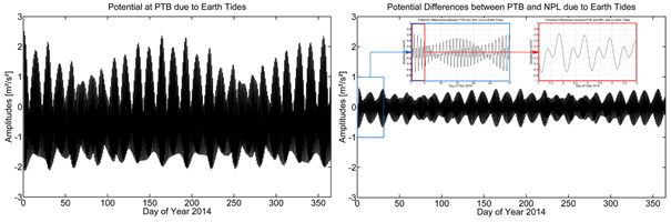
Fig 1: Gravitational potential at the Earth's surface due to the solid Earth tides at PTB (left) and
corresponding potential differences between PTB and NPL (right) in the year 2014; units are m²/s²
Regarding the oceans, the mass fluctuations associated with the ocean tides cause a direct attraction effect of the corresponding water masses, which would lead to a change in the potential even on a rigid Earth, and a distortion of the Earth due to the loading effect. All these induced signals are called the 'load tides', which combine with the body tides to make up the total tides.
Similar to the external tidal forcing, the ocean tidal loading effects as well as the effects of other surface mass loads can be computed by corresponding load Love numbers h', l', k', but opposite to the solid Earth tides, the load Love numbers are required up to high degrees (e.g. nmax = 10000), and also their dependence on the degree n is important. Related to the Earth's surface, again a combination of the load Love numbers in the form (1 + k' - h') is relevant, and finally the summation over all degrees yields the entire potential effect.
Fig 2 shows the gravitational potential at the Earth's surface due to the ocean tides for station PTB (top left) and NPL (top right) as well as corresponding potential differences between PTB and NPL (bottom) in the year 2014. It is clear that the ocean tide effects depend strongly on the distance to the coast, and global maximum values are found at the French and British Atlantic coasts. The amplitudes at NPL are about 0.3 m2/s2 (about 10–15 % of the solid Earth tides), while the corresponding potential difference signal is smaller with amplitudes below 0.15 m2/s2.
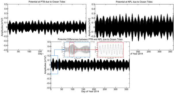
Fig 2: Gravitational potential at the Earth's surface due to ocean tides at PTB (top left) and NPL (top right),
as well as corresponding potential differences between PTB and NPL (bottom) in the year 2014; units are m²/s²
Besides the Earth's body and ocean load tides, tidal variations also result from the atmosphere (atmospheric tides), polar motion (solid Earth and ocean pole tides) and variations in the angular velocity of the Earth (length of day tides).
Non-tidal mass redistributions
Besides the tidal signals, the gravity potential of the Earth is also affected by non-tidal mass redistributions within the atmosphere, hydrosphere, cryosphere, and geosphere, inducing again direct gravitational effects as well as deformations (loads) associated with additional potential effects. For instance, non-tidal mass variations in the atmosphere occur due to atmospheric pressure and other variations on daily to yearly scales, atmospheric pressure conditions and strong wind effects lead to non-tidal mass redistributions in the oceans, and further effects are related to continental hydrology changes, solid Earth processes, etc.
Summary
The solid Earth tides contribute the by far largest time-variable component of the gravity potential with amplitudes up to about 3 m2/s2 in the considered examples, while ocean tide effects are roughly 10 % smaller than the solid Earth tides. All other effects are again roughly one order of magnitudes smaller than the ocean tides, and hence are negligible in many cases. Further details on the topic of time-variable gravity potential components for optical clock comparisons and international timescales will be given in an upcoming separate publication.
The research within this EURAMET joint research project receives funding from the European Community's Seventh Framework Programme, ERA-NET Plus, under Grant Agreement No. 217257.